In this post I am going to try to answer the questions above. Regarding the first question, I’ll explain where the question began for me. Then, I will review the meaning of the terms Variance and Standard Deviation, and review the basic steps in Analysis of Variance (ANOVA). Finally, I’ll show how I think ANOVA can be extended to two dimensions, and, to address the second question, show why the whole process, was a big bust.
Can Analysis of Variance be generalized to multi-dimensions? That is the question that I’ve been mulling lately, and making random facebook posts in my angst the last week or so.
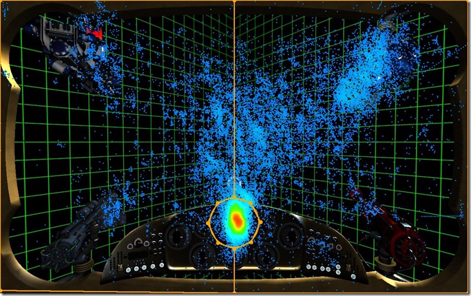
The question comes from my eye-data heat maps. The two figures below show where people look on the screen during my video-game task. Each point is a record of looking at that spot on the screen. The brighter / hotter colored points indicate more looks accumulating over time in that area.
The top figure is one group, the bottom is a different group, treated differently. The difference in how they were treated is not important. 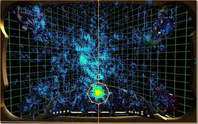
Ignore the hot spot in the circle. When not looking in the circle, it is pretty clear to me that the groups are looking at the screen differently. The bottom group tends to look to the right, particularly up at the weapon while the top group tends to look around on the left side of the screen.
To analyze something like these patterns the screen is divided up into regions (a priori preferably) and the number of looks (or time spent looking) by each subject in each region is counted and analyzed.
I thought it would be nice to take the raw data themselves, the XY coordinate pairs, and determine if the groups differ in where they are looking when not looking in the circle.
Individually, it would be a (relatively) simple matter to determine if the groups differ in their average X coordinates, or average Y coordinates. I could simply do two separate analyses of variance, one on X, and one on Y.
When you do an analysis of variance, you compare the variance within groups of scores to the variance between groups of scores. The idea is that if everything is random, the variance within a group of scores should be the same as the variance between a group of scores.
That is… Between Variance / Within Variance = 1.
Variance is a statistic used to estimate variability, how much numbers tend to change. It is calculated simply. A score, X, is subtracted from the Mean of the scores, that difference is squared, that is done for every number, and all of those are added up and divided by N-1. The variance is the average squared difference from the mean
Sum( X- MeanX)^2 / N – 1
The first part of the equation
Sum (x-MeanX)^2
is called the Sum of Squares, or SS. It is the sum of squared deviations around the mean.
The denominator, N-1, is called the “degrees of freedom” or DF. I’ll talk more about degrees of freedom further down. (there are good reasons to use N-1 here instead of N that have to do with estimating populations- stuff that we don’t need to get into here).
The square root of the variance is called the standard deviation. It is something very similar to the average deviation of a score from the mean- not exactly though, (the sqrt of the average of squares is not the same as the average of the sqrt of squares) but close enough.
In the end, the standard deviation
Sqrt( Sum (X-MeanX)^2 / N-1 )
and the Absolute deviation
sum( abs(X-MeanX))/N)
are almost always linearly related where Standard deviation = 1.253314137 * Absolute deviation.
Why all the squaring? Why not just work with absolute differences?
The answer some might give is “It gets rid of negative numbers” which is a simple-minded answer people give either because they are ignorant, or don’t feel like the student is ready for the real reason.
Truth be told, I’m somewhat on the ignorant side. I really do not fully follow the sum total of the real reasons- in part it has to do with some esoteric, but important, arguments between Fisher and Eddington. You can get into those meaty reasons here if you are so inclined.
Now me, I like to make up my own reasons and state them with reason and authority so they appear to make sense and are not challenged.
I have always thought of the squaring as having to do with Pythagoras.
C = sqrt( A^2 + B^2)
The length of the hypotenuse of a triangle is equal to the square root of the sum of the squares of each leg.
If you have a point at X1,Y1, and another point at X2,Y2, the length of A is X1-X2 and the length of B is Y1-Y2.
C = sqrt((X1-X2)^2+(Y1-Y2)^2)
So, assume you only have one variable, drop Y, and you have
C = sqrt(X1-X2)^2
do that for a bunch of X points, substituting MeanX for X2, and you are just calculating the sum of squares, and begin to see the standard deviation emerging. The standard deviation relates differences to distances, at least in my mind.
Now, back to ANOVA. Suppose you have two groups of numbers and want to know if they differ more than you’d expect by chance. You could do an ANOVA (given many assumptions..).
| .99 | 1.73 |
| .78 | 2.11 |
| .4 | 1.92 |
| 3.07 | 3.87 |
| -.24 | .37 |
The first thing we would do is begin calculating all our sums of squares. We start considering all the numbers together as one big group.
Sum of Squares total = SS Total = Sum(X-GM)^2 where GM =Grand Mean. GM = 1.5
SStotal = 14.98
Next, we’d calculate the Sum of squares for each group-
Sum(X-Lm)^2 where Lm = Local group mean. The mean for the first group is 1, and that for the second group is 2.
SSgroup1 = 6.23 and for SSgroup2 = 6.25. Add them together and we get 12.48
Next, we would calculate the Sum of Squares between the groups. To do that, we use the means and take the size of the groups into account.
SSbetween = sum( n * (lm-Gm)^2) where n is the size of the group which is being compared to the grand mean.
SSbetween = 5*(1-1.5)^2+5*(2-1.5)^2 = 2.5
Now we collect N-1 for all the sums of squares to use in the divisions to create variances.
Total we have 10 numbers, 9 degrees of freedom.
Within the first group we have 5 numbers, so 4 degrees of freedom, same for the second group, so we have 8 degrees of freedom within our groups.
We have two groups, so we have 1 degree of freedom between our groups. Lets arrange all that into the standard ANOVA summary table.
| Sum of Squares | DF | Variance | F | P | |
| Between | 2.5 | 1 | 2.5 | 1.60 | .24 |
| Within | 12.48 | 8 | 1.59 | ||
| Total | 14.98 | 9 |
Notice that between + within = total, and that is as it should be. Now, we’d divide each SS by its relevant DF and get the variances for Within and Between, then divide between by within to get F.
F says that the variance between the groups is 1.6 times bigger than the variance within a group. With a little Excel magic (Fdist()) we can say that would happen with a probability of .24 just by chance. We really don’t have any evidence that the groups are different.
Lets now imagine that we had measured the groups on a separate variable, Y. The data for Y look like…
| 2.18 | 3.55 |
| .71 | 1.36 |
| 2.41 | 2.35 |
| .11 | 2.36 |
| -.42 | 4.59 |
The mean for the first group is 1 and the mean for the second is 2.84. If we then do an analysis of variance we would obtain the following.
| SS | DF | Variance | F | P | |
| Between | 8.5 | 1 | 8.5 | 5.44 | .048 |
| Within | 12.5 | 8 | 1.56 | ||
| Total | 21 | 9 |
With Y, we have 5.44 times as much variance between the groups as we have within the groups- and that would happen with a probability of .048 by chance. We are reasonably safe in saying that the groups are different. They are significantly different, so to speak.
Now imagine both variables, X and Y together.
| Group 1 | Group 2 | |||
| Scores | X | Y | X | Y |
| .99 | 2.18 | 1.73 | 3.55 | |
| .78 | .71 | 2.11 | 1.36 | |
| .4 | 2.41 | 1.92 | 2.35 | |
| 3.07 | .11 | 3.87 | 2.36 | |
| -.24 | -.42 | .37 | 4.59 | |
| Means | 1 | 1 | 2 | 2.84 |
| Standard Deviations | 1.25 | 1.25 | 1.25 | 1.25 |
Group 1 forms a cluster of points at x=1, y=1 with a standard deviation (~average distance from the mean) of 1.25.
Group 2 forms a cluster of points at x=2, y=2.84, with a standard deviation of 1.25.
You might imagine, as I did, those two point clusters as the following diagram. Each circle is centered at a group mean and has a radius of 1.25. When I began to do that, I got excited. Would it not be nice to be able to analyze the two clusters as a whole using ANOVA. It seemed to make sense to me.
Why would it be nice? Well I thought- look at the overlap when you just consider X
There is a lot of X overlap, thus it is no wonder we were unable to conclude that the groups were different when looking only at X.
Now look at the overlap in Y-
There is much less overlap in Y, thus, we were able to conclude that yes, we do have two different groups of numbers here.
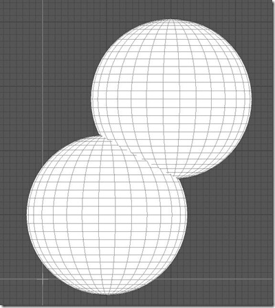
But look at the amount of overlap when X and Y are considered together-
Not much overlap at all there- if we could test the differences based on both dimensions at once, we should have a more powerful test, as there is clearly less overlap.
The hypotenuse is longer than either leg, always.
That glorious thought is what made me believe the analysis would be more powerful. But it turns out to be the problem that I did not consider, that ultimately burst my balloon. I had to go through the steps to get there, so I’m not letting you off the hook with the punchline- let us proceed.
How might this ANOVA be done. Its all Pythagoras I thought. Don’t work with differences, work with distances.
Rather than compute sums of squares beginning with the square of the difference from the mean of the variables, one variable at a time, compute the sums of squares as the square of the distance from the mean of the points.
Remember Pythagoras from above…
C = sqrt( A^2 + B^2)
…where A and B are the lengths of the legs of the triangle, computed as the difference between two points.
C = sqrt( (X1-X2)^2+(Y1-Y2)^2)
One of our points will simply always be a mean, the grand mean of points, or the mean of points in each group.
The Grand mean of points would be the mean of the X coordinates and the mean of the Y coordinates, or (1.5, 1.92).
Sum of squares total would be
sum( ( x – GMx)^2 + (y – GMy)^2 )
If we do that, we get SS Total of 35.98.
Then, we’d get SS Within- where we do
sum( (x-Lmx)^2 +(y-Lmy)^2)
for each group and add those together and we’d get 24.98.
Finally, we’d do the sum of squares for Between. Expanding our equation we’d have
sum (n1*(LmX-GMx)^2+n2*(LmY – GMy)^2)
And we’d get 11.
Now, we need to get our degrees of freedom. Degrees of freedom tell you how many numbers are free to vary. I have 4 numbers in my head. That’s all I’ve told you, and given that, I can change any or all of the 4 numbers- it makes no difference to you. But, if I tell you the numbers average 6, then I am no longer free to change the numbers willy nilly. I can change 3 of them, but the fourth must be something specific to obtain a mean of 6. When you describe a group of numbers, you lose a degree of freedom.
In our one-variable ANOVA we had 9 degrees of freedom total. But now we are analyzing two variables together, so would we have 18? 9 for the X, and 9 for the Y? The answer is no- we would still have 9. Each XY combination describes a point, and if either X or Y change, the point is different. So, there are not double the degrees of freedom.
Our summary table would look like the following:
| SS | DF | Variance | F | P | |
| Between | 11 | 1 | 11 | 3.52 | .097 |
| Within | 24.98 | 8 | 3.12 | ||
| Total | 35.98 | 9 |
There are two things that got my attention here. The sums of squares are just the sums of squares from the X analysis added those from the Y analysis. After looking at the formula, I had a “duh” reaction, as the formula simply add the squared deviations for X to those for Y.
But, my next reaction was the F. The variance between the groups of points is 3.52 times as much as the variance within a group of points, and that would happen with a probability of .097 by chance- we could not conclude that the groups are significantly different.
What gives? The analysis of Y said the distributions were different, and the figures show that there is less overlap between the distributions when both variables are considered at once. The F here should be bigger than in the analysis of Y alone, and the P should have been smaller.
Take the square root of the within variance in the analysis above. It is 1.77. What that is saying is that the standard deviation of the distances is 1.77. The standard deviation of the differences among either X or Y alone was 1.25.
I drew the circles with a radius of 1.25, but that wasn’t right. The average difference in the X direction was 1.25, and the average difference in the Y direction was 1.25, thus, the standard deviations describe the length of the legs of a triangle. The radius of the circle would be the hypotenuse.
R = sqrt (1.25^2+1.25^2) = 1.77
So, the circles should have really been drawn as below.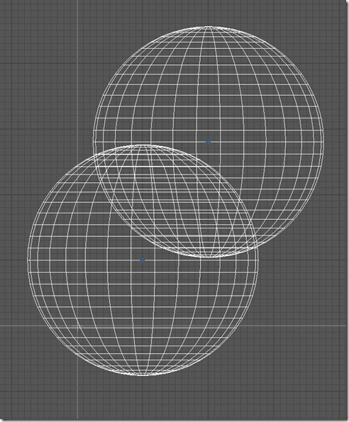
Now, the overlap is considerable.
How can that be I wondered- how can the standard deviation of X or Y be changing depending on the other variable? The X and Y extents overlap considerably more than in the earlier figures.
When we only consider X, we are collapsing across Y. When we only consider Y we are collapsing across X. Given the circular distributions extreme values of X get less frequent with extreme values of Y, and vice versa. So, when we collapse across either variable we are increasing the frequency of probable values more so than the frequency of improbable values. Thus, the distributions get more peaked, and the standard deviation gets smaller.
Consider the two distributions below.
3 3
2 3 4 2 3 4
1 2 3 4 5 1 2 3 4 5
Each has a standard deviation of 1.22.
Now, group them together (collapse over whatever distinguishes he two distributions) and you’d have
3
2 3 4
2 3 4
1 2 3 4 5
1 2 3 4 5
and you’d have a standard deviation of 1.18.
In summary, I think ANOVA can be extended to 2 variables by working with distances rather than differences, but you wouldn’t want to because the hypotenuse is always longer than the legs, thus the overlap in the distributions will be larger when both variables are considered together in a Euclidian combination than considered alone.
Of course, this might all be completely innacurate BS, but thats the best I can do with it. I’m a psychologist Jim, not a statistician..
What I need for my heatmaps is some more sophisticated cluster analyses, such as the Ordering Points to Identify Clustering Structure algorithm. I’ve neither the time nor knowledge resources at the moment to begin that, but I see it coming in the future.

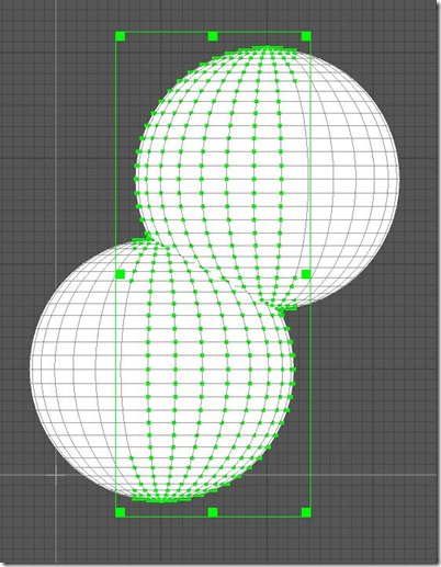
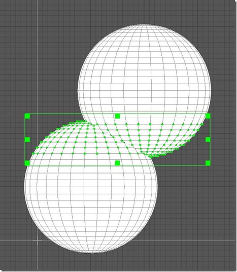
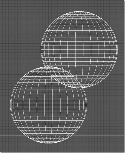
From centroid, in terms is distances and direction (in radians?), points can be described.
I don’t understand a thing, but keep sending these. I am interested in what you are doing.
Some old horse . . .
And why not to raise it by means of a MANOVA better than an ANOVA?
On the other hand, for the analysis of the frequency of fixings, us we are raising a log-linear analysis (i.e. glm in R software: glm(Fr.Cx~Stim*Trial, family = poisson, data= ExtracCx)).
MANOVA is also less powerful than ANOVA, and geometrically I’m less able to reason out exactly what is being analyzed with everything represented as matrices.
Don’t the observations have to be independent for the log linear analysis? Frequency of fixations on a screen can’t be independent because the areas are mutually exclusive of each other over time. When you are looking in one area, you can’t be looking in others.
Then the model of measure is like in the analysis of correspondences, where the categories that the observers evaluate are mutually exclusive, rightly as one of the areas with more log-linear work. In addition this is only like that if the area where the subjects are looking is an independent variable but not if only we want to compare the frequency of fixings in a particular area. Also they exist log-linear for models of dependence and even analogous to ARIMA with autocorrelation.
In MANOVA there would be analyzed the Variate, that would be a linear combination of the measures in variable dependent paths. What is included in this linear combination does not depend on MANOVA but of the dependent chosen variable, which might be a spatial measure equally. The advantage that I see him is that it goes rightly to the heart of the question, to analyze that one that is common to the dependent variables.
I realize what MANOVA does- Once the relevant sums of squares matrices are calculated their determinants are found and F is constructed from a ratio of determinants. There are multiple ways that the F can be determined as well- introducing more experimenter flexibility (i.e., greater Type 1 error) into the analysis.
The F will tell you that some linear combination of X and Y produces differences- but then you must extract that equation and determine if it makes any sense with regards to the data and the question.
Also, MANOVA works best when DVs are correlated, and there is no reason for X & Y coordinates to have any correlation with each other in a heat map.
I haven’t read this properly, but would circular ANOVA be any use to you here?
I’d never heard of circular anova- but after reading up a bit on directional statistics I don’t think it’d gain me much as the analysis would only consider the angular deviations of the centroids from some central point, without taking into consideration their distances from each other. -as I understand it (which is very limited).
Possibly. I think if you use some sort of analyses with the von mises distribution you’ll deal with this issue though “Given the circular distributions extreme values of X get less frequent with extreme values of Y, and vice versa”
(i’ve read it more carefully now!)
Pingback: Visualizing effect sizes, the effect of N, and significance. | Byron's blog.
Reblogged this on Just another complex system.
Hi,
I would like to propose the link exchange deal with your website drjbn.wordpress.com, for mutual benefit in getting more traffic and improve search engine’s ranking, absolutely no money involve.
We will link to you from our Fashion and Women authority site – https://www.souledamerican.com/, from its homepage’s sidebar. In return you will agree to do the same to link back to one of our client site, from your drjbn.wordpress.com’s homepage too (sidebar, footer, or anywhere on your homepage), with our brand name Harajuku Fever.
If you are interested, kindly reply to this email.
Thank you,
Charles